Recreating the Talent vs Luck Model

I recently came across the paper titled Talent vs Luck: the role of randomness in success and failure, by A. Pluchino. A. E. Biondo, A. Rapisarda, on Hacker News on Hackernews. After reading through both the Scientific American and checking out the paper itself, I decided to try and recreate the model to learn more about it and follow up on some questions I had about the paper’s findings.

I go over my opinions on the paper’s findings in this companion post.

In this post, I first review the model as I understand it, demonstrate how I was able to recreate it, and show that the results from my recreation have roughly the same features as the one in the paper. As a disclaimer, I should note that I had not used Netlogo before this, and wasn’t able to find all of the possible Netlogo constraints in the paper. My model is likely not identical to the one in the paper, but does use same the dynamics and has similar results. If anyone finds errors in the code or in this post, please let me know in the comments or open a PR on the Github repo.

Model Explainer

The paper employs agent-based modelling using Netlogo. Netlogo models are based on simulating interactions between things called “agents” that are placed into a 2D space where they can move and interact over time. Where they are placed, and how they move & interact are configurable parts of any model.

One great sample model that helps illuminate this is the Wolf Sheep Predation model. In this model, the 2D space represents the habitat that both animal populations live in. On setup, the wolf and sheep are placed randomly onto the space. Then on each step through time, wolf & sheep can move around, procreate, or hunt/be hunted, and die. As the model runs, it shows how the size of the two groups trends over time.

The model proposed in this paper features three different agents: people (black), lucky events (green), and unlucky events (red). At the outset, all three agents are distributed onto the 2D space at random. Here’s a screenshot of the initial setup shown in the paper:

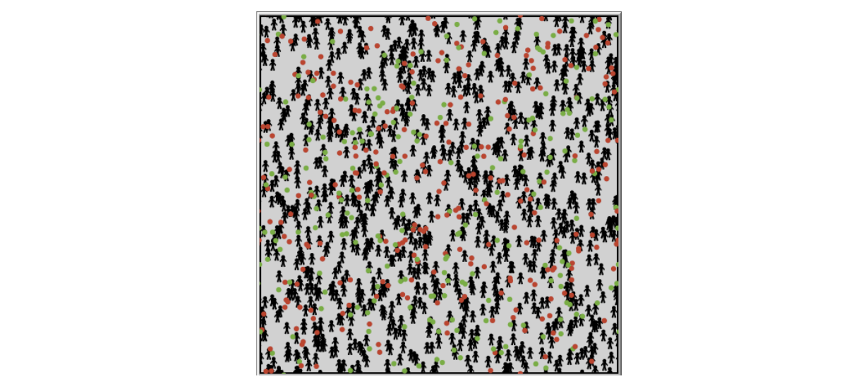
The model proceeds in steps through time, during which event points move around randomly. The researchers aimed to model a 40 year career in 6-month segments, or 80 steps through time. People start with the same allotment of capital, and are given a number between 0 and 1 to represent their “talent”. Talent is normally distributed.

As I understand it, the way people acquire or lose capital occurs between each step, and depends on whether the person has come into contact with an event point as follows:

1. The person intercepted no events, and their capital doesn’t change value.
2. The person intercepted a lucky event, and the agent doubles their capital if their talent number exceeds a randomly generated number between 0 and 1.
3. The agent intercepted an unlucky event, and the agent halves her capital.

Rewriting in NetLogo

With Netlogo, there are two main sections in which you develop your model: the Interface tab, and the Code tab. The Interface tab is where the visualization of the environment is. This is also the place where you build out GUI inputs for a model. The Code tab is where the core model is specified. The code is a little finniky to learn how to write, and basically has to follow the DSL that NetLogo defines for getting the model set up and running.

From the model’s description in the paper, we know the following constraints:

1. There should be 1000 people with normally distributed talent, 250 lucky events, and 250 unlucky events.
2. The events should move around at random.
3. People should gain or lose capital when they intercept events.
4. The model should play out over 80 steps, representing a 40 year working life.

Based on this, we can define our model’s setup in NetLogo:

extensions [csv]

globals [capital-list talent-list]
breed [ lucky-events lucky-event ]
breed [ unlucky-events unlucky-event ]
breed [ people person ]
turtles-own [ xc yc ]
people-own [capital talent outlist ]

to setup
  clear-all

  create-lucky-events initial-number-lucky-events
  [
    set shape  "dot"
    set color green
    set size 2  ; easier to see
    set label-color blue - 2
    setxy random-xcor random-ycor
  ]
  create-unlucky-events initial-number-unlucky-events
  [
    set shape  "dot"
    set color red
    set size 2  ; easier to see
    set label-color red - 2
    setxy random-xcor random-ycor
  ]

  create-people initial-number-people
  [
    set shape "person"
    set color brown
    set size 3  ; easier to see
    set capital initial-capital
    set talent random-normal mean-talent talent-std-dev
    set outlist []
    setxy random-xcor random-ycor
  ]
  display-labels
  reset-ticks
end

Without going into the detail, the basics of the above are that we’re creating three types of agents in the model: the lucky and unlucky events, and the people. This setup refers back to inputs for the initial numbers of these agents, the mean talent and standard deviation desired, and so on. All of these are placed randomly onto the initial map.

The step-by-step changes in the model are defined similarly:

to go
  if ticks >= career-length * 2 [
    export-capital-vals
    stop
  ]
  ask lucky-events [
    move
  ]
  ask unlucky-events [
    move
  ]
  ask people [
    if people-move [ move ]
    interact-with-events

    set outlist list (talent) (capital)
  ]
  tick
  display-labels
end

The basics here are that in each run, we ask the events to move. We also can optionally make people move. Then the key part: we ask the people to interact with events on their same patch of the 2D space. The basic event interaction is defined as:

to interact-with-events-persistent
  if count (lucky-events-here) >= 1 and (talent > random 1)
    [ set capital capital * 2 ]
  if count unlucky-events-here >= 1
    [ set capital capital / 2 ]
end

With this, we now have encoded the basic model dynamics from the paper. For the full code, I encourage readers to go to the Github repo and check it out.

As a note, there are a number of factors that I could not find in the paper:

1. The size of the 2D space, and its patch size
2. The distance and “randomness” that goes into the events moving
3. Whether people also move (it seems like they don’t, but just for fun I’ve made it an option in my model)
4. Whether events disappear after someone takes advantage of them.

As I don’t know the answers for what the paper’s authors did here, I’ve tried to account for that in my model. In it, it’s possible to toggle whether to have events die after being used, and whether people move. There are also inputs for how far events move with each step. As for the environment size, it’s definitely seems clear that varying the size of the environment changes the concentration of capital quite dramatically.

Running the model

To run the model I’ve built, download Netlogo and the talent-vs-luck.nlogo file from my repo. Then open the Netlogo model on your computer. You should see a screen like this:

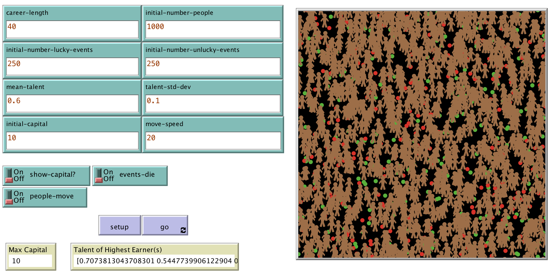
After that, press “Setup” and then “Go”. Feel free to change any inputs you like.

The model is built to output some information on the screen, and other information onto an output.csv file from the directory where it was run.

Comparing results

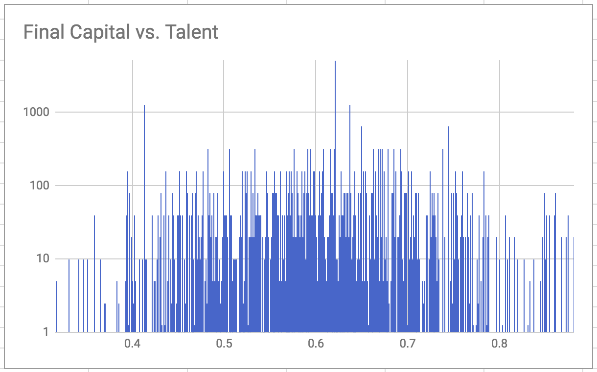
I built out a spreadsheet to analyze the results from my model, and compare them back to the paper’s results. One of my first runs with a working model yielded a max capital of 5120, by a person with a near-to-average talent of 0.62. I uploaded these results into this Google spreadsheet (feel free to make a copy of it for your own use). As with the paper, the initial raw results show capital success quite distributed across talent:

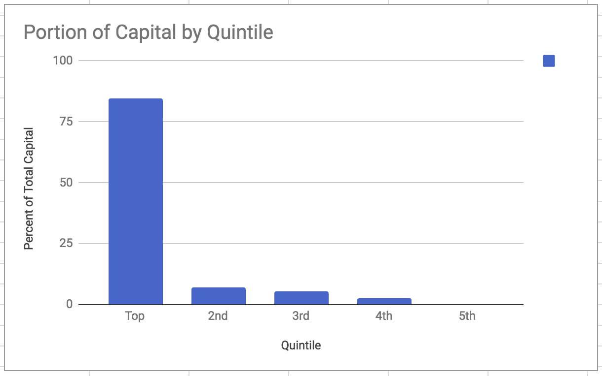
To be sure that this run has similar features as described, I looked into how much capital was held by the upper quintile, finding that roughly 80% of the capital was held by the top:

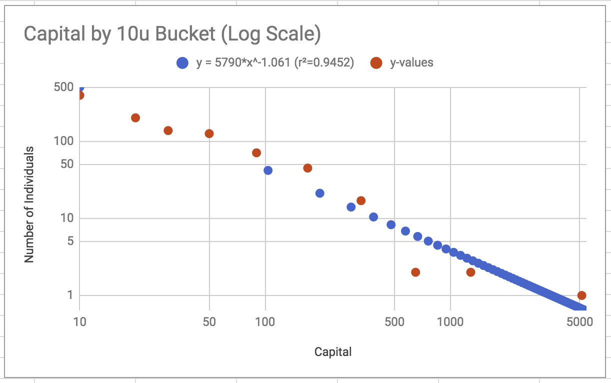
I also found that a similar power-law feature could be found in how capital was held. The paper’s results had a power closer to -1.3, vs this run’s -1.06, but I’m going to assume that’s not too big of a deal.

Conclusion

For the most part, I think my model yields results that roughly align with the features described in the paper. As I mentioned earlier, there are a number of constraints that I didn’t find described in the paper, and without them it’s hard to be sure how close my setup is to theirs.

Most significantly, I’ve noticed that changing the environment size does lead to much higher max capital accumulations, but also a far higher concentration of capital (closer to 95% capital held by the top 20% in some runs). Meanwhile, the setup I used for my results above uses a space size 80x80, and leads to lower max capital accumulations, but generally uploads the 80-20 rule better. It would be interesting to know if the researchers from the paper found the same, and what constraints they used for these unspecified parts of their model.

After building this out myself, and reviewing both my own results and the paper in more depth, I’ve written up a post on my opinions of the paper. You can read that here.

Here’s a link to the Github Repo, if you want to check out the code and/or run it yourself.

Here’s a link to the spreadsheet used to analyze results from the model.